The Vašulka Live Archive website is a learning environment for exploring the work of Steina and Woody Vasulka in terms of recurring visual and audio motifs, through the use of expert artificial neural networks and specially designed website features and interfaces.
The machine learning method of Convolutional Neural Networks (CNN) (LeCun et al., 1989) was used in the project to formally, quantitatively analyze and statistically validate art-historians’ knowledge and theories related to the visual and acoustic iconography of the Vašulkas' work. Two expert artificial neural networks [AI software tools] have been developed that are able to search a database of videos from the work of Steina and Woody Vašulka for predefined, pictorial and audio objects. The Neural Networks determine the range of occurrence of these objects relative to the time of the video, and express in statistical terms the degree of probability with which a given object is identified by the neural network. In order to effectively use these intelligent tools, an original web-interface [Machine Learning] has been designed, while the [Machine Vision] section of the web serves a didactic function as it introduces visitors to how the perceptual apparatus of artificial intelligence works in the process of analysis of artistic videos by the Vašulkas.
The machine learning method of Convolutional Neural Networks (CNN) (LeCun et al., 1989) was used in the project to formally, quantitatively analyze and statistically validate art-historians’ knowledge and theories related to the visual and acoustic iconography of the Vašulkas' work. Two expert artificial neural networks [AI software tools] have been developed that are able to search a database of videos from the work of Steina and Woody Vašulka for predefined, pictorial and audio objects. The Neural Networks determine the range of occurrence of these objects relative to the time of the video, and express in statistical terms the degree of probability with which a given object is identified by the neural network. In order to effectively use these intelligent tools, an original web-interface [Machine Learning] has been designed, while the [Machine Vision] section of the web serves a didactic function as it introduces visitors to how the perceptual apparatus of artificial intelligence works in the process of analysis of artistic videos by the Vašulkas.
Dataset
An important input parameter in the development of intelligent software is the dataset, on which the artificial neural networks are trained. In the case of the Vašulka Live Archive project, these are videos by Steina and Woody Vašulka, stored in a digital archive managed by the Centre for New Media Arts - Vašulka Kitchen Brno. The total volume of the archive is 536 GB and at the time of the project's launch its content consisted mostly of uncatalogued or otherwise organized audiovisual, visual and textual material of various types.Therefore, when preparing the dataset, we first identified digital objects whose extensions suggested that they were audiovisual works. Specifically, the extensions were: ifo, vob, mpg, mpeg, rec, dir, mob, san, dav, mov, avi, ppj, swf, dad, wp3, mp4, prproj, flc and fli. Out of a total of 1,800 audiovisual works, we successfully converted 880 video files to mp4 video files using the h.264 codec. The remaining 920 files could not be converted (they were, for example, objects with the mob extension). The resulting set of successfully converted videos created a data corpus of 137 GB, which included 1 252 items that would take six days, 20 hours and 27:30 minutes to watch. However, not all of these videos were created by the Vašulkas’, and many of the Vašulkas' videos, in turn, appeared repeatedly in the archive, in varying length, quality, and format.
The unprocessed archive first had to be organized in the traditional way. This means identifying the works of the Vašulka family and creating a database of them, which can be navigated according to defined categories. By comparing online archives and lists of the Vašulkas’ works on websites (Vasulka.org, Foundation Langlois, LI-MA, Electronic Art Intermix, Berg Contemporary, Monoskop.org), a complete list of Vasulka's works was created for this purpose. In this way we identified a total of 108 titles, 21 by Woody and 49 by Steina Vašulka, and 38 titles by the Vašulkas together. We were able to track down a total of 105 unique works by the Vašulkas’ in the Vašulka Kitchen Brno archive. We can therefore claim that this is an almost complete collection of audiovisual works, which includes art videos, video-documentations of installations and documentaries, most of which are represented in their complete versions and some of which are available at least as fragments. In total, the Vašulka Live Archive website contains approximately 200 videos.
Based on our research of the above archives and considering the specifics of the Vašulkas' work, we have created a list of categories that we have assigned to the individual videos (Table 1). At the basic level, the videos were organized using standard metadata descriptions - author/author, title, year, artistic medium. We have also added more detailed descriptions of the videos – names of collaborators, names of video protagonists, names of tools and their authors, and annotations that briefly describe the work itself. Like many other video artists, the Vašulkas’ reused their works repeatedly, in different splices, or integrated them into multi-monitor and spatial installations, which they often conceived of as stand-alone works. A filmic terminology (prequel, sequel and quotation) was used to describe these relationships. Another feature of the Vašulkas’ work is the integration of videos into larger units (e.g. Studies, Sketches), which can also be traced on the web.
| Primary identifiers: | author, other author(s), title of the work, year of creation |
| Identifiers of the relationships of videos to each other: | series, prequel, sequel, quote |
| Identifiers of the technical solution and the used medium: | artistic medium, technical medium, applied tools and software |
| Summary of video content: | annotation, performers |
At this stage of the project, the project team needed a shared workspace for collaborative work on video description (cataloguing) and tagging (object identification). The corpus of audiovisual works and the corresponding predefined categories were therefore imported into a specially programmed web interface. Once the work on the description of the individual works and the tagging of the videos was completed, the dataset was ready for training for the artificial neural networks.
Visual and sound objects
The list of categories of sound and image motifs that can be searched for in the Vašulkas' work was compiled by a team of art historians based on the identification of objects that emerge throughout the Vašulkas' work and are thus rightly considered to be the bearers of recurring content and, in part, formal motifs in their work. The list of categories was iterated gradually during the project considering the neural network results. The final list of object classes is presented in an alphabetical list (see Table 2).| Visual classes | Audio classes | |
| Air | Landscape | Acoustic music |
| Body | Letter | Air (noise) |
| Car | Machine vision | Car (noise) |
| Digit | Rutt/Etra scan processor | Electronic music |
| Earth | Steina | Fire (noise) |
| Effect | Stripes | Noise |
| Face | TV set | Speech |
| Fire | Violin | Violin playing |
| Interior | Water | Vocal music |
| Keying | Woody | Water (noise) |
From the point of view of the iconography of the Vašulkas' work, however, a simple listing of the categories searched is insufficient. In fact, there are several groups of pictorial and sound symbols (see Table 3).
| Thematic clusters | Visual objects |
| Human | Body, Face, Steina, Woody |
| Interier/exterier | Interier, Landscape* |
| Natural elements | Air, Earth, Fire, Water |
| Special electrical signal manipulation effects | Rutt/Etra processor, Keying, Machine vision (fisheye effect), Effect |
| Machine and tool | Car, TV, Violin |
| Symbols | Digit, Letter, Lines |
* The binary opposition of interior/exterior allowed to categorize the videos according to whether they are gallery installations or recordings of studio work, or whether they are shots of natural and urban landscapes.
Like the pictorial classes, the classes of sound objects form higher units in terms of the iconography of Vasulka's work. These are usually pandans to visual categories, or designations of binary oppositions, for example between the recording of natural sound and the noise of manipulated electronic media (Table 4).
| Thematic clusters | Audio objects |
| Human | Speech, Singing |
| Tools | Electronic Music, Noise, Acoustic Music, Playing Violin |
| Natural elements | Air (noise), Water (noise), Fire (noise) |
| Machines | Car (noise) |
Machine Learning
Given that the dataset, in the form of the Vašulkas’ videos, has very specific visual and audio qualities related both to the topics being processed and to the characteristic use of special effects in the manipulation of the electronic signal, we can conclude that the developed intelligent software is a completely unique tool for the iconographic (audio and video) analysis of early video art, specifically that of Steina and Woody Vašulka. Each of these AI-tools can be used independently, i.e. we can track the occurrence of specific visual or audio objects across videos. The added value, however, is the ability to use both tools and thus work with the outputs of both software's work when analyzing videos. This is encouraged by the very audio-visual nature of video art, and thus the frequent representation of objects by visual and audio signifiers simultaneously. Using the outputs of both tools makes it possible to observe how the representation of objects by visual or audio signifiers is mutually supportive in these audio-visual works (Fig. 1) or how visual and audio objects convey a dominant position within the audiovisual experience (Fig. 2).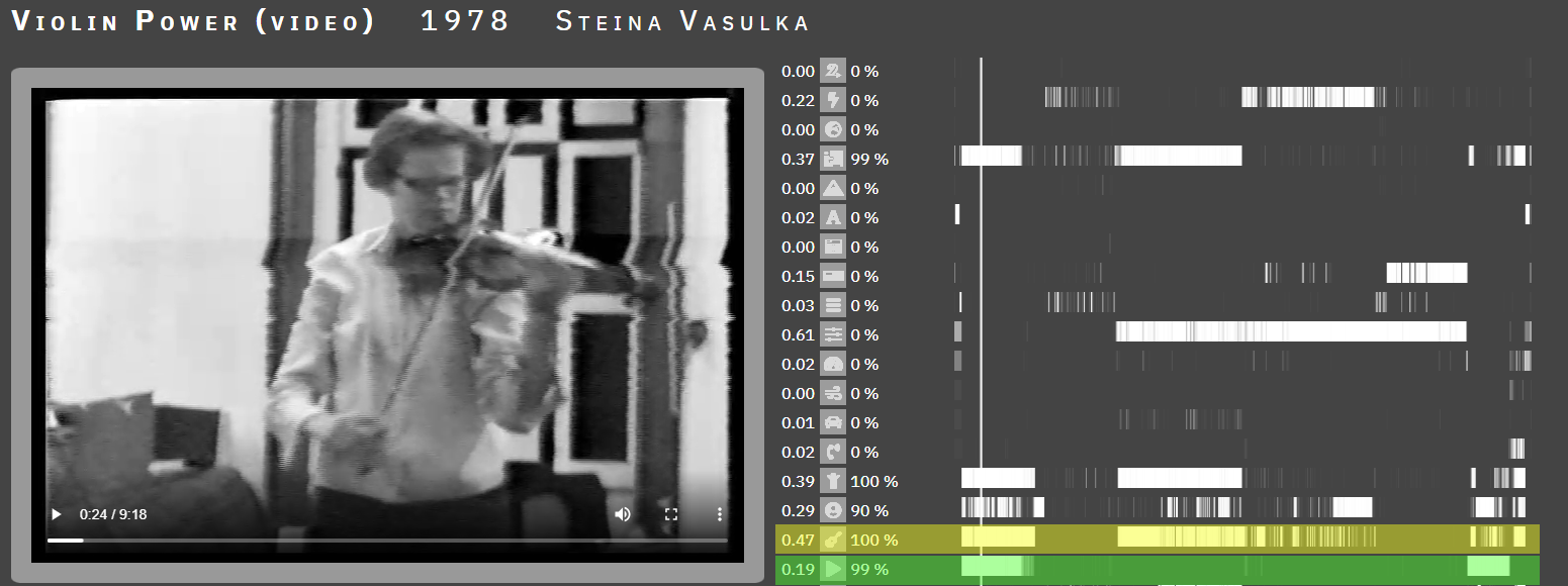
In Figure 1, the visual predictions of the violin are shown in yellow and the auditory predictions of the violin are shown in green. The figure shows that the image contains a violin and the neural network correctly predicts 100 % of the occurrences of violins in the image. Since the audio track clearly contains the sound of violin playing, the neural network correctly predicts 99 % of the occurrence of this sound.
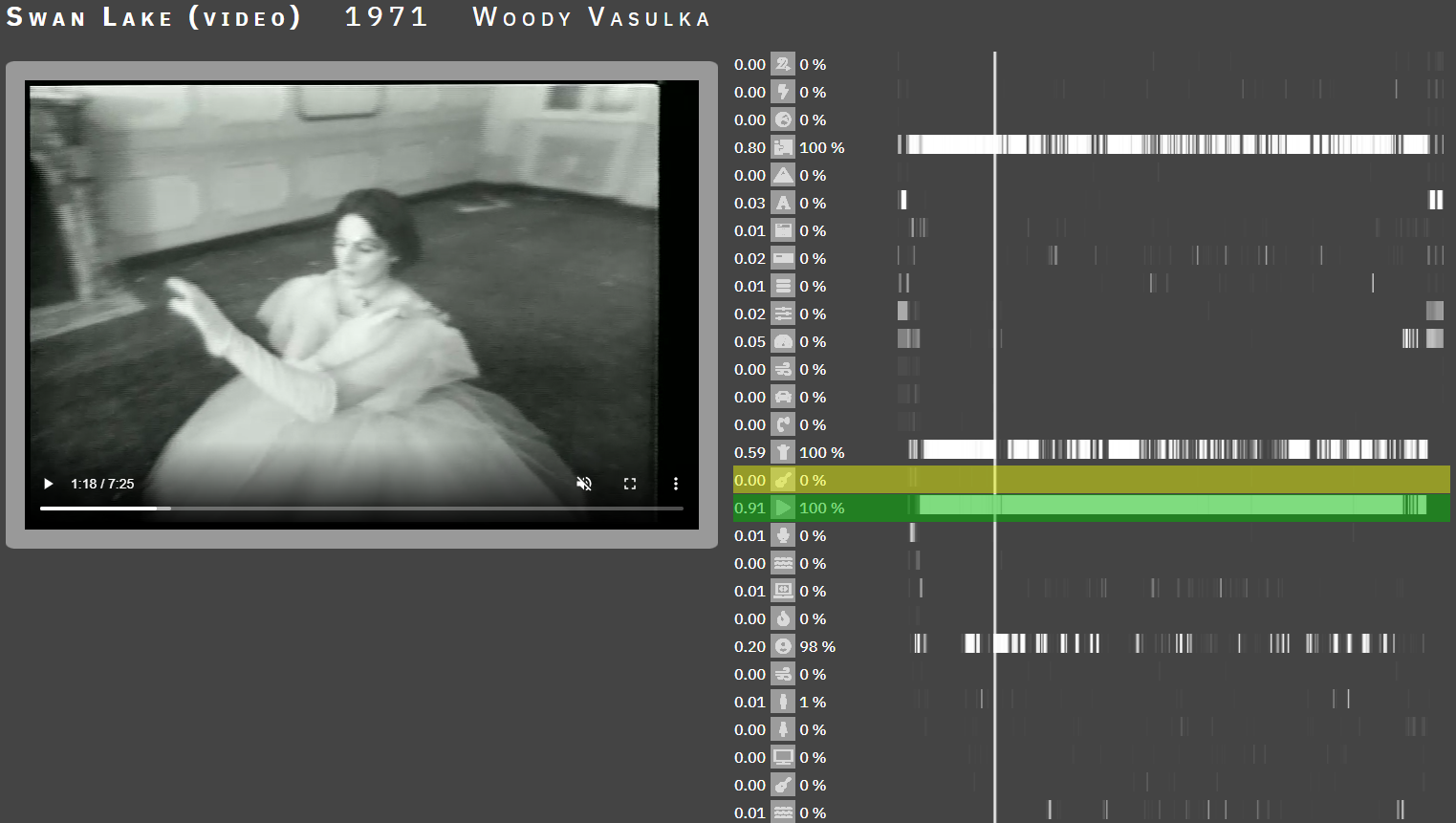
In Figure 2, the visual predictions of the violin are again marked in yellow and the audio predictions in green. This piece contains violin playing in 91 % of its length in the audio track. In contrast, the violin is not visually present in the demonstration.
The above examples of both software working show how both tools can be used in the analysis of audiovisual works. Together, the software for audio and video recognition forms an adequate tool for content analysis of Vašulkas’ audio-visual works.
Machine learning – web design
For the Machine Learning section, a web interface was designed with several functionalities that allow not only to search and view individual videos stored in the Vašulkas’ database, but especially to study the iconography of the Vašulkas' work across the archive of their videos using the results of artificial neural networks.
At a basic level, the videos on the site are organized using standard metadata descriptions (see Table 1). In addition, the site provides several unique functional interfaces that have been designed to convey information obtained using specially developed software tools to web users. For example, the site allows the Vašulka videos to be filtered by the frequency of occurrence of each visual and audio feature in each video, with frequencies calculated as the percentage of occurrences of a given feature in the video frames with a probability threshold of 1%. The equation is as follows:
Suppose we have a video V, an element E1 (a vector of probabilities per frame), and a probability threshold P = 1%:
F = number of frames in V
H = number of frames where E1 >= P
Weight E1 at P = H / F
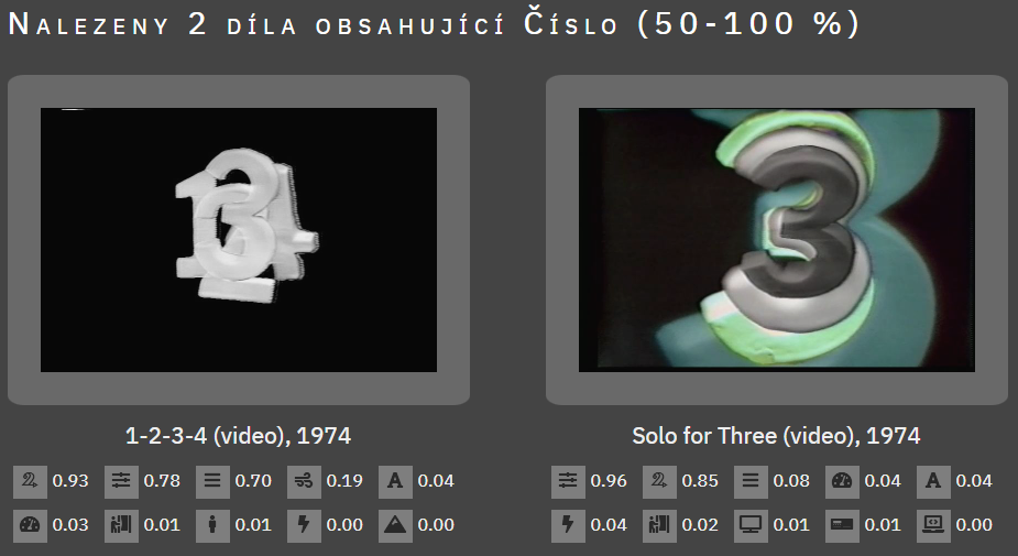
For example, in the video 1-2-3-4.mp4 (Steina and Woody Vašulka, 1974), the element Number was identified in 93 % of the frames and thus the weight is 0.93. However, the range of element weights searched is optional and can be reduced to 1 %. This feature allows searching for videos that contain the selected element or a combination of several elements across the database, even videos in which the occurrence of the object is minimal are not excluded from the selection. This feature not only makes the site an effective search tool, but also increases the rigor of the argument and may lead to new findings about Vašulkas’ work that have so far escaped the attention of art historians.
Figure 3 shows an example listing the videos after selecting the highest threshold, 50-100 %, for the Number feature. From the enumeration, it can be seen that there are two videos in the entire database containing the Number element in at least 50 % of the frames of the entire video.
Video classification results can be studied frame by frame. The video player is complemented by a control panel that displays a list of defined video and audio features, including data on their frequency of occurrence based on a weight (with per-video precision) and a probability measure (with per-frame precision). As the video plays, the cursor automatically moves on timelines leading horizontally from each category. However, it is also possible to rewind the video by moving the cursor along this axis. This functionality is shown in Figures 1 and 2.
The identified similarities between the videos, obtained through exact image and sound analysis using AI-software, are expressed on the web as the result of calculating the "distances" between the videos, each represented by a vector of weights. It is assumed that if the distance between two videos is small, then there is a high degree of similarity between them, and vice versa. For this purpose, two different standard algorithms have been tested: Manhattan distance and cosine similarity (Pandit & Gupta, 2011). Finally, Manhattan distance was used to recommend similar videos to the currently playing video in the Machine Learning/Machine Learning section. This is because this distance metric is computationally inexpensive and also proved to be suitable for content-based retrieval.
Machine Vision
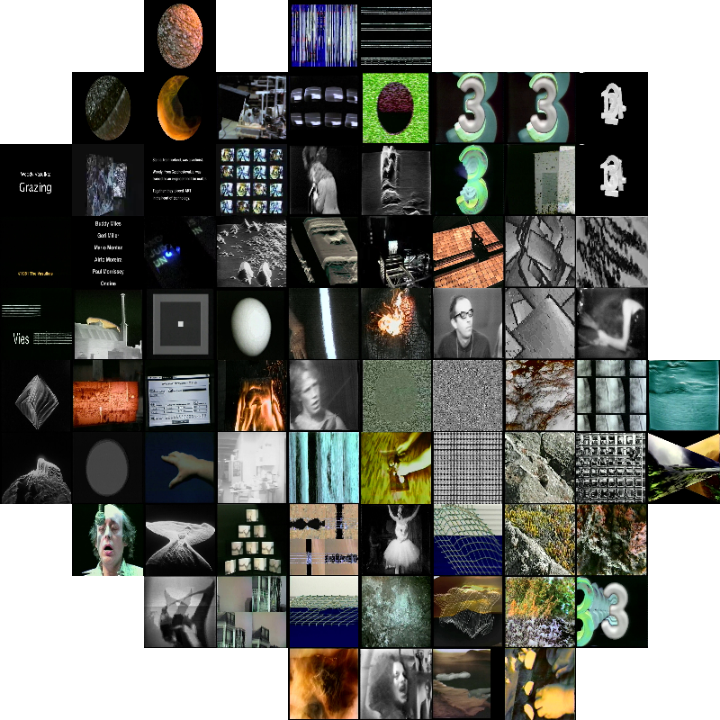
On the Machine Vision page, we focused on conveying the view of artificial intelligence, i.e. how an artificial neural network works in the process of perceiving the creation of Vašulkas’ work. We were inspired to incorporate it into the architecture of the site by the Activation Atlas project, which visualizes the neural network functions in the different layers of the artificial neural network in the perception process (Carter et al., 2019), aiming to convey to a wider audience an understanding of how this widespread and powerful technology of today works.Karpathy (2014) used outputs from a fully connected layer of a convolutional neural network, which he then plotted into a 2D map using the t-SNE algorithm (van der Maaten & Hinton, 2008). The t-SNE tool allows the reduction of hard-to-imagine multidimensional spaces into commonly used 2D and 3D spaces. The computations result in a grid layout of the images in which the items are arranged such that their locations correspond to their similarity to each other. We used our re-trained convolutional neural network model called Xception (Chollet, 2017) for visualization. The model was presented with frames from Vašulkas’ videos as input, which were pre-selected using an algorithm programmed by us. The algorithm adequately selected the frames so as not to create duplicates by selecting each frame from all videos. These frames were fed into the model input to obtain unique flags for each frame from a layer called add 3. These outputs were then reduced to 2D coordinates using the t-SNE algorithm. The resulting rendering of the images using this procedure is shown in Figure 4.
The creators of the Activation Atlas have added new functionality to this two-dimensional, static visualization that provides a view of how the neural network recognizes certain visual objects in the corresponding dataset. The authors accomplished this by inverting the activation visualization flags from the image classification network, thus allowing observation of how the artificial neural network typically represents certain features of the processed images.
Unlike other ways of representing the outputs of neural network work, which give us results in the form of a list of recognized items and a measure of the probability of their occurrence in a given image, the dynamic interface of Activation Atlas offers a more comprehensive view of the work of intelligent software that better matches reality, i.e., how neural networks "see" visual objects. Indeed, in practice, artificial neural networks very rarely search for a single, isolated item (class), but usually several items are searched for simultaneously, making the whole process and its results much more complex.
The creators compare the benefits of the Activation Atlas to the situation when we try to describe how writing works in the case of natural language. While t-SNE provides us with a basic familiarity with the workings of artificial neural networks, which can be likened to discovering that the Latin alphabet is made up of 26 letters (and English 42 letters, as it includes letters with accents), Activation Atlas is a tool that allows us to observe different combinations of artificial CNN neurons, which in the case of language is equivalent to being able to observe how these letters are used to form words. The dynamic interface thus contributes much more to the understanding of how language works, in this case the language of artificial intelligence.
Activation Atlas makes use of the Lucid library ( Lucid, 2018) to create the visualizations themselves. In our project, this library was used to create visualizations for the Vasulka dataset, which were then applied to the layout described in the previous chapter. The results are shown in Figure 5.
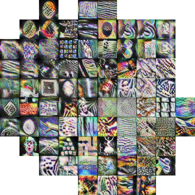
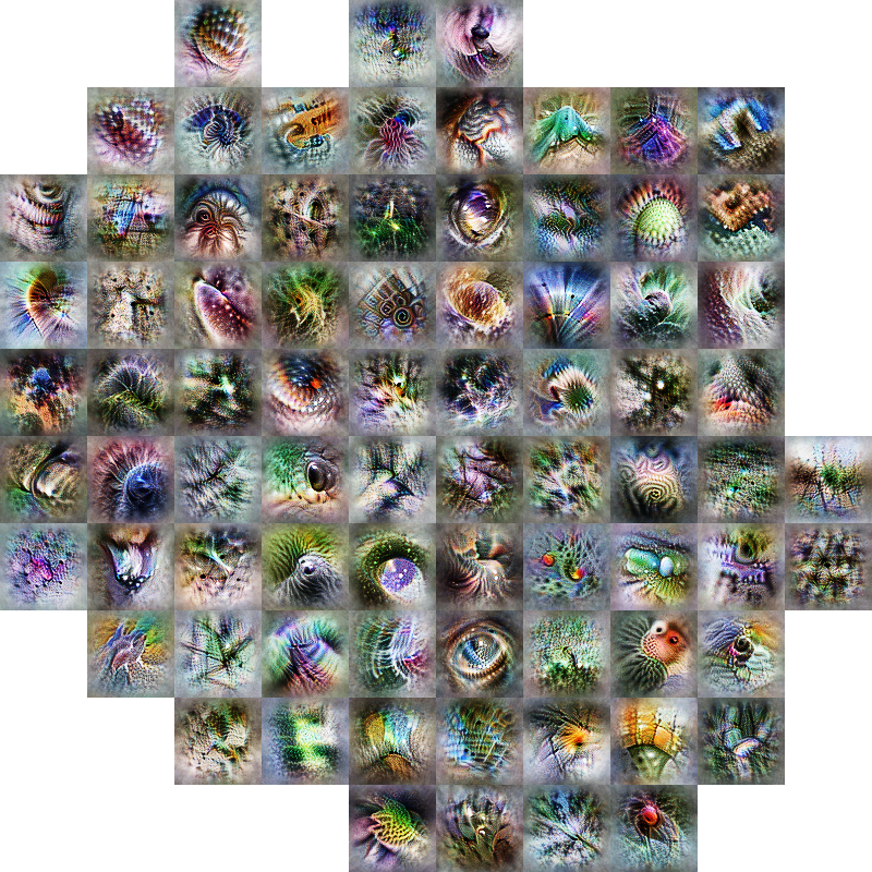
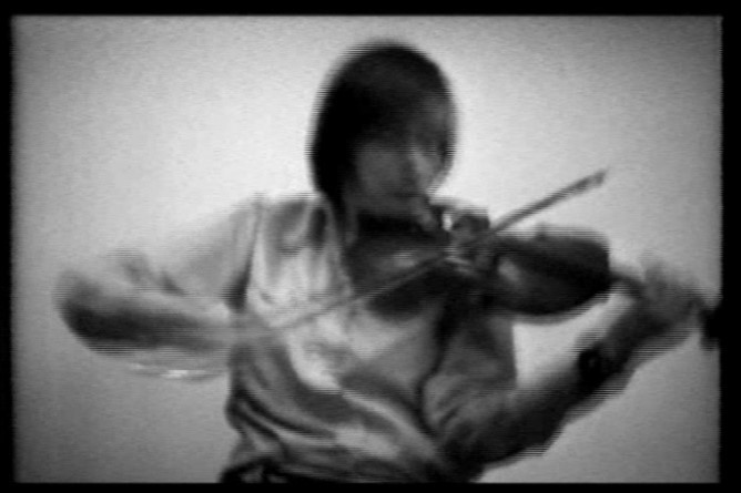
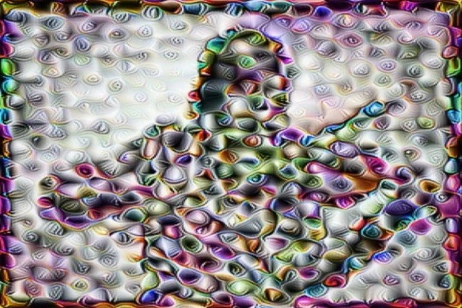
Figure 6 is a screenshot from the Violin Power video (1978, Woody and Stein Vasulka) from second 17 (left) and its visualization using the Lucid library (right).
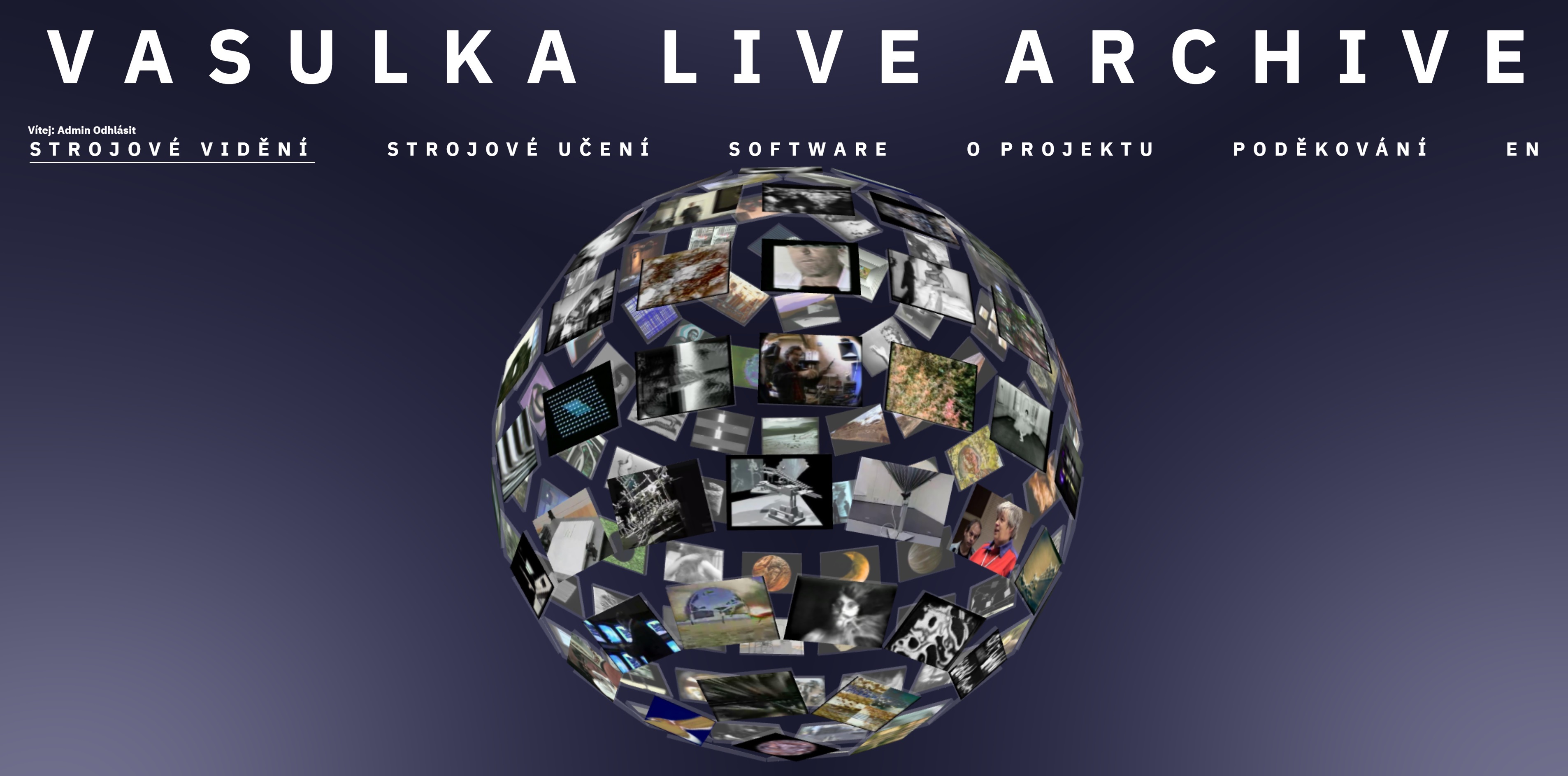
The contribution of Machine Vision lies in its didactic function. It allows to observe how neural networks work in the process of a pseudo-perception of the Vašulkas’ artistic videos. In contrast to the 2D layout of Activation Atlas, in our project the representation of machine vision is created using the JavaScript library Three.js (Cabello, 2010) and based on the use of a sphere shape onto which selected images from the Vašulkas’ videos have been mapped. An example of the resulting sphere is shown in Figure 7, left. The shape of the sphere is one of the characteristic visual motifs and a functional tool associated with the concept of machine vision in the Vašulkas’ work. The mirror sphere is symbolically placed in the centre of the optical apparatus of Machine Vision (Steina Vašulka, 1978) or Allvision (Steina Vašulka 1976) and in combination with cameras recording the image of the surroundings reflected in its mirrored surface, it achieves an extension of the field of view of the human eye, i.e. the spectrum visible to humans. To the same end, the Vašulkas’ also used the convex shape of the "fisheye" effect to evoke the expanded perspective of the machine's view (see, for example, Steina Vasulka: Summer Salt, 1982).
Steina Vašulka wrote about this: “In the late seventies, I began a series of environments titled Machine Vision and Allvision, with a mirrored sphere. … These automatic motions simulate all possible camera movements freeing the human eye from being the central point of the universe.” (Steina Vašulka: Machine Vision)
When you hover your mouse over any of the images, you will first see a list of objects that have been recognised by the AI with a certain probability. When we click on an image, the layers of the artificial neural network are spread out in front of us, where we can observe how the neural network's analytical eye gradually decomposes and analyses it, so that at the end of the process a report of what it "sees" is issued in the form of a label of the relevant categories and a percentage of the probability of the result. The decomposed neural network layers for the snapshot from Techne and Eros (Stein and Woody Vašulka, 1999) are shown in Figure 8.
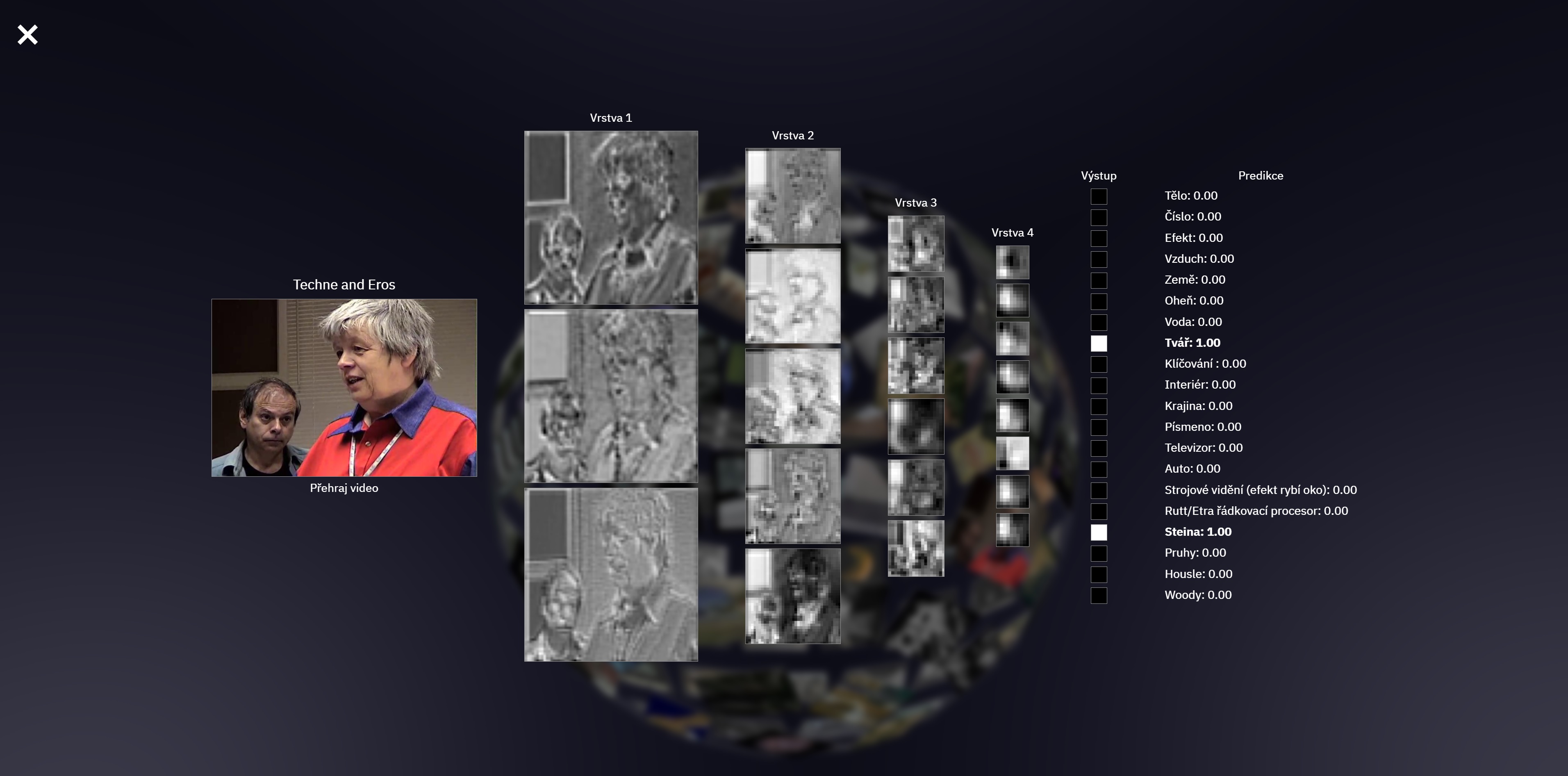
Similarly to the Activation Atlas project, our project uses the principle of neural networks to represent the processes of neural networks. Out of 132 layers, only five layers were selected for clarity, but they sufficiently illustrate the decomposition of the image to capture the image features. Thanks to these unique image features, it is then possible to identify individual objects and thus predict their appearance in a given image.
AI Software Tools
The source code of the trained neural networks has been deposited on GitHub, which serves as a repository for the results of software engineering research projects. GitHub was launched in 2008 and was founded by Tom Preston-Werner, Chris Wanstrath and PJ Hyett. It is a platform that promotes community collaboration in software engineering using the Git versioning tool.The software for the image and the software for the sound are hosted HERE.
Both neural networks are published in open source, under the MIT license.
Please credit the origin if used:
Sikora, P. (2022). MediaArtLiveArchive – Video Tagging [Software]. https://github.com/vasulkalivearchive/video
Miklanek, S. (2022). MediaArtLiveArchive – Audio Tagging [Software]. https://github.com/vasulkalivearchive/audio
References
Cabello, R. (2010). Three.js – Javascript 3D Library. Three.js. https://threejs.org/Carter, S., Armstrong, Z., Schubert, L., Johnson, I., & Olah, C. (2019). Activation Atlas. Distill, 4(3). https://doi.org/10.23915/distill.00015
Chollet, F. (2017, July). Xception: Deep Learning with Depthwise Separable Convolutions. 2017 IEEE Conference on Computer Vision and Pattern Recognition (CVPR). https://doi.org/10.1109/cvpr.2017.195
Karpathy, A. (2014). t-SNE visualization of CNN codes. Andrej Karpathy Academic Website. https://cs.stanford.edu/people/karpathy/cnnembed/
LeCun, Y., Boser, B., Denker, J. S., Henderson, D., Howard, R. E., Hubbard, W., & Jackel, L. D. (1989). Backpropagation Applied to Handwritten Zip Code Recognition. Neural Computation, 1(4), 541–551. https://doi.org/10.1162/neco.1989.1.4.541
Lucid. (2018). [Software]. https://github.com/tensorflow/lucid
Pandit, S., & Gupta, S. (2011). A Comparative Study on Distance Measuring Approaches for Clustering. International Journal of Research in Computer Science, 2(1), 29–31. https://doi.org/10.7815/ijorcs.21.2011.011
van der Maaten, L., & Hinton, G. (2008). Visualizing Data using t-SNE. Journal of Machine Learning Research, 9(86), 2579–2605. http://jmlr.org/papers/v9/vandermaaten08a.html
Vasulka, S. (?). Machine Vision. Vasulka.org. http://www.vasulka.org/Steina/Steina_MachineVision/MachineVision.html